Automatic Hyperparameter Tuning - A Visual Guide (Part 1)

Selecting the right hyperparameters can make or break your machine learning model. But who has time for endless trial and error or manual guesswork? Luckily, automatic hyperparameter tuning is there to the rescue.

By cleverly sampling the search space and pruning unpromising trials early, automatic tuning can help you find the best hyperparameter settings quickly and effortlessly. Plus, it frees you up to focus on other important tasks, like drinking coffee or napping ;). As a personal and concrete example, I used this technique on a real elastic quadruped to optimize the parameters of a controller directly on the real robot.

In this blog post, I’ll explore some of the techniques for automatic hyperparameter tuning, using reinforcement learning as a concrete example. I’ll discuss the challenges of hyperparameter optimization, and introduce different samplers and schedulers for exploring the hyperparameter space. In part two (WIP), I’ll show how to use the Optuna library to put these techniques into practice.

If you prefer to learn with video, I recently gave this tutorial at ICRA 2022. The slides, notebooks and videos are online:

Hyperparameter Optimization: The “n vs B/n” tradeoff

When you do hyperparameter tuning, you want to try a bunch of configurations “n” on a given problem. Depending on how each trial goes, you may decide to continue or stop it early.

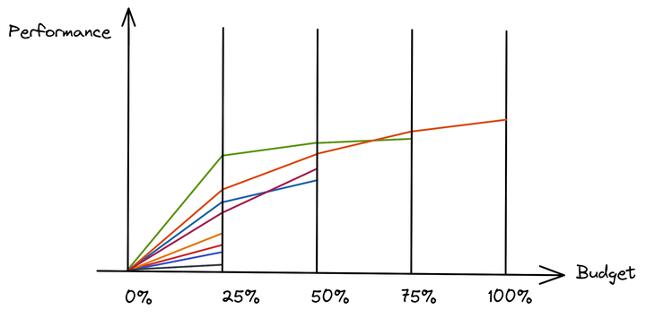
The tradeoff you have is that you want to try as many configurations (aka sets of hyperparameters) as possible, but you don’t have an infinite budget (B). So you have to allocate the budget you give to each configuration wisely (B/n, budget per configuration).

As shown in the figure above, one way to achieve this goal is to start by giving all trials the same budget. After some time, say 25% of the total budget, you decide to prune the least promising trials and allocate more resources to the most promising ones.

You can repeat this process several times (here at 50% and 75% of the maximum budget) until you reach the budget limit.

The two main components of hyperparameter tuning deal with this tradeoff:

• the sampler (or search algorithm) decides which configuration to try
• the pruner (or scheduler) decides how to allocate the computational budget and when to stop a trial

Samplers

So how do you sample configurations, how do you choose which set of parameters to try?

The Performance Landscape

Let’s take a simple 2D example to illustrate the high-level idea.

In this example, we want to obtain high returns (red area). The performance depends on two parameters that we can tune.

Of course, if we knew the performance landscape in advance, we wouldn’t need any tuning, we could directly choose the optimal parameters for our task.

In this particular example, you can notice that one parameter must be tuned precisely (parameter one), while the second one can be chosen more loosely (it doesn’t impact performance much). Again, you don’t know this in advance.

Grid Search

A common and inefficient way to sample hyperparameters is to discretize the search space and try all configurations: this is called grid search.

Grid search is simple but should be avoided. As shown in the image above, you have to be very careful when discretizing the space: if you are unlucky, you might completely miss the optimal parameters (the high return region in red is not part of the sampled parameters).

You can have a finer discretization, but then the number of configurations will grow rapidly. Grid search also scales very poorly with dimensions: the number of configurations you have to try grows exponentially!

Finally, you may have noticed that grid search wastes resources: it allocates the same budget to important and unimportant parameters.

A better but still simpler alternative to grid search is random search.

Random Search

Random search samples the search space uniformly.

It may seem counterintuitive at first that random search is better than grid search, but hopefully the diagram below will be of some help:

By sampling uniformly, random search no longer depends on the discretization, making it a better starting point. This is especially true once you have more dimensions.

Of course, random search is pretty naive, so can we do better?

Bayesian Optimization

One of the main ideas of Bayesian Optimization (BO) is to learn a surrogate model that estimates, with some uncertainty, the performance of a configuration (before trying it). In the figure below, this is the solid black line.

It tries to approximate the real (unknown) objective function (dotted line). The surrogate model comes with some uncertainty (blue area), which allows you to choose which configuration to try next.

A BO algorithm works in three steps. First, you have a current estimate of the objective function, which comes from your previous observations (configurations that have been tried). Around these observations, the uncertainty of the surrogate model will be small.

To select the next configuration to sample, BO relies on an acquisition function. This function takes into account the value of the surrogate model and the uncertainty.

Here the acquisition function samples the most optimistic set of parameters given the current model (maximum of surrogate model value + uncertainty): you want to sample the point that might give you the best performance.

Once you have tried this configuration, the surrogate model and acquisition function are updated with the new observation (the uncertainty around this new observation decreases), and a new iteration begins.

In this example, you can see that the sampler quickly converges to a value that is close to the optimum.

Gaussian Process (GP) and Tree of Parzen Estimators (TPE) algorithms both use this technique to optimize hyperparameters.

Other Black Box Optimization (BBO) Algorithms

I won’t cover them in detail but you should also know about two additional classes of black box optimization (BBO) algorithms: Evolution Strategies (ES, CMA-ES) and Particle Swarm Optimization (PSO). Both of those approaches optimize a population of solutions that evolves over time.

Now that you’re familiar with the different samplers for automatic hyperparameter tuning, it’s time to dive into another critical aspect: pruners. These techniques work hand in hand with the search algorithms to further improve the efficiency of the optimization process.

Schedulers / Pruners

The job of the pruner is to identify and discard poorly performing hyperparameter configurations, eliminating them from further consideration. This ensures that your resources are focused on the most promising candidates, saving valuable time and computating power.

Deciding when to prune a trial can be tricky. If you don’t allocate enough resources to a trial, you won’t be able to judge whether it’s a good trial or not.

If you prune too aggressively, you will favor the candidates that perform well early (and then plateau) to the detriment of those that perform better with more budget.

Median Pruner

A simple but effective scheduler is the median pruner, used in Google Vizier.

The idea is to prune if the intermediate result of the trial is worse than the median of the intermediate results of previous trials at the same step. In other words, at a given time, you look at the current candidate. If it performs worse than half of the candidates at the same time, you stop it, otherwise you let it continue.

To avoid biasing the optimization toward candidates that perform well early in training, you can play with a “warmup” parameter that prevents any trial from being pruned until a minimum budget is reached.

Successive Halving

Successive halving is a slightly more advanced algorithm. You start with many configurations and give them all a minimum budget.

Then, at some intermediate step, you reduce the number of candidates and keep only the most promising ones.

One limitation with this algorithm is that it has three hyperparameters (to be tuned :p!): the minimum budget, the initial number of trials and the reduction factor (what percentage of trials are discarded at each intermediate step).

That’s where the Hyperband algorithm comes in (I highly recommend reading the paper). Hyperband does a grid search on the successive halving parameters (in parallel) and thus tries different tradeoffs (remember the “n” vs. “n/B” tradeoff ;)?).

Conclusion

In this post, I introduced the challenges and basic components of automatic hyperparameter tuning:

• the trade-off between the number of trials and the resources allocated per trial
• the different samplers that choose which set of parameters to try
• the various schedulers that decide how to allocate resources and when to stop a trial

The second part (WIP) will be about applying hyperparameter tuning in practice with the Optuna library, using reinforcement learning as an example (if you are impatient, the video and the colab notebook are already online).

Acknowledgement

All the graphics were made using excalidraw.

Did you find this post helpful? Consider sharing it 🙌