Getting SAC to Work on a Massive Parallel Simulator: An RL Journey With Off-Policy Algorithms (Part I)

This post details how I managed to get the Soft-Actor Critic (SAC) and other off-policy reinforcement learning algorithms to work on massively parallel simulators (think Isaac Sim with thousands of robots simulated in parallel). If you follow the journey, you will learn about overlooked details in task design and algorithm implementation that can have a big impact on performance.

Spoiler alert: quite a few papers/code are affected by the problem described below.

• Part I is about identifying the problem and trying out quick fixes on SAC.
• Part II (WIP) will be about tuning SAC for speed and making it work as good as PPO.

A Suspicious Trend: PPO, PPO, PPO, …

The story begins a few months ago when I saw another paper using the same recipe for learning locomotion: train a PPO agent in simulation using thousands of environments in parallel and domain randomization, then deploy it on the real robot. This recipe has become the standard since 2021, when ETH Zurich and NVIDIA¹ showed that it was possible to learn locomotion in minutes on a single workstation. The codebase and the simulator (called Isaac Gym at that time) that were published became the basis for much follow-up work².

As an RL researcher focused on learning directly on real robots, I was curious and suspicious about one aspect of this trend: why is no one trying an algorithm other than PPO?³ PPO benefits from fast and parallel environments⁴, but PPO is not the only deep reinforcement learning (DRL) algorithm for continuous control tasks and there are alternatives like SAC or TQC that can lead to better performance⁵.

So I decided to investigate why these off-policy algorithms are not used by practitioners, and maybe why they don’t work with massively parallel simulators.

Why It Matters? - Fine Tuning on Real Robots

If we could make SAC work with these simulators, then it would be possible to train in simulation and fine-tune on the real robot using the same algorithm (PPO is too sample-inefficient to train on a single robot) .

By using other algorithms it might also be possible to get better performance. Finally, it is always good to have a better understanding of what works or not and why. As researchers, we tend to publish only positive results, but I think a lot of valuable insights are lost in our unpublished failures.

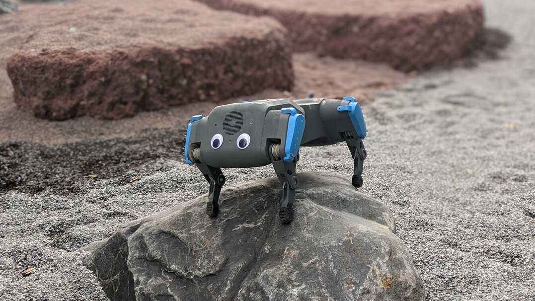
The DLR bert elastic quadruped

(The Path of Least Resistance) Hypothesis

Before digging any further, I had some hypotheses as to why PPO was the only algorithm used:

• PPO is fast to train (in terms of computation time) and was tuned for the massively parallel environment.
• As researchers, we tend to take the path of least resistance and build on proven solutions (the original training code is open source and the simulator is freely available) to get new interesting results⁶.
• There may be some peculiarities in the environment design that favor PPO over other algorithms. In other words, the massively parallel environments might be optimized for PPO.
• SAC/TQC and derivatives are tuned for sample efficiency, not fast wall clock time. In the case of massively parallel simulation, what matters is how long it takes to train, not how many samples are used. They probably need to be tuned/adjusted for this new setting.

Note: during my journey, I will (obviously) be using Stable-Baselines3 and its fast Jax version SBX.

The Hunt Begins

There are now many massively parallel simulators available (Isaac Sim, Brax, MJX, Genesis, …), here, I chose to focus on Isaac Sim because it was one of the first and is probably the most influential one.

As with any RL problem, starting simple is the key to success.

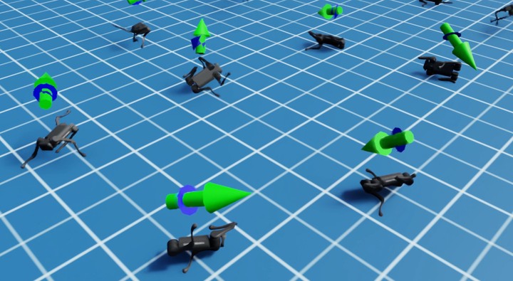
A PPO agent trained on the Isaac-Velocity-Flat-Unitree-A1-v0 locomotion task.
Green arrow is the desired velocity, blue arrow represents the current velocity

Therefore, I decided to focus on the Isaac-Velocity-Flat-Unitree-A1-v0 locomotion task first, because it is simple but representative. The goal is to learn a policy that can move the Unitree A1 quadruped in any direction on a flat ground, following a commanded velocity (the same way you would control a robot with a joystick). The agent receives information about its current task as input (joint positions, velocities, desired velocity, …) and outputs desired joint positions (12D vector, 3 joints per leg). The robot is rewarded for following the correct desired velocity (linear and angular) and for other secondary tasks (feet air time, smooth control, …). An episode ends when the robot falls over and is timed out ( truncation) after 1000 steps⁷.

After some quick optimizations (SB3 now runs 4x faster, at 60 000 fps for 2048 envs with PPO), I did some sanity checks. First, I ran PPO with the tuned hyperparameters found in the repository, and it was able to quickly solve the task. In 5 minutes, it gets an average episode return of ~30 (above an episode return of 15, the task is almost solved). Then I tried SAC and TQC, with default hyperparameters (and observation normalization), and, as expected, it didn’t work. No matter how long it was training, there was no sign of improvement.

Looking at the simulation GUI, something struck me: the robots were making very large random movements. Something was wrong.

SAC out of the box on Isaac Sim during training.

Because of the very large movements, my suspicion was towards what action the robot is allowed to do. Looking at the code, the RL agent commands a (scaled) delta with respect to a default joint position:

# Note desired_joint_pos is of dimension 12 (3 joints per leg)
desired_joint_pos = default_joint_pos + scale * action

Then, let’s look at the action space itself (I’m using ipdb to have an interactive debugger):

import ipdb; ipdb.set_trace()
>> vec_env.action_space
Box(-100.0, 100.0, (12,), float32)

Ah ah! The action space defines continuous actions of dimension 12 (nothing wrong here), but the limits $[-100, 100]$ are surprisingly large, e.g., it allows a delta of +/- 1432 deg!! in joint angle when scale=0.25, like for the Unitree A1 robot. To understand why normalizing the action space matters (usually a bounded space in $[-1, 1]$), we need to dig deeper into how PPO works.

PPO Gaussian Distribution

Like many RL algorithms, PPO relies on a probability distribution to select actions. During training, at each timestep, it samples an action $a_t \sim N(\mu_\theta(s_t), \sigma^2)$ from a Gaussian distribution in the case of continuous actions⁸. The mean of the Gaussian $\mu_\theta(s_t)$ is the output of the actor neural network (with parameters $\theta$) and the standard deviation is a learnable parameter $\sigma$, usually initialized with $\sigma_0 = 1.0$.

This means that at the beginning of training, most of the sampled actions will be in $[-3, 3]$ (from the Three Sigma Rule):

The initial Gaussian distribution used by PPO for sampling actions.

Back to our original topic, because of the way $\sigma$ is initialized, if the action space has large bounds (upper/lower bounds » 1), PPO will almost never sample actions near the limits. In practice, the actions taken by PPO will even be far away from them. Now, let’s compare the initial PPO action distribution with the Unitree A1 action space:

The same initial Gaussian distribution but with the perspective of the Unitree A1 action space $[-100, 100]$

For reference, we can plot the action distribution of PPO after training⁹:

Distribution of actions for PPO after training (on 64 000 steps).

The min/max values per dimension:

>> actions.min(axis=0)
array([-3.6, -2.5, -3.1, -1.8, -4.5, -4.2, -4. , -3.9, -2.8, -2.8, -2.9, -2.7])
>> actions.max(axis=0)
array([ 3.2,  2.8,  2.7,  2.8,  2.9,  2.7,  3.2,  2.9,  7.2,  5.7,  5. ,  5.8])

Again, most of the actions are centered around zero (which makes sense, since it corresponds to the quadruped initial position, which is usually chosen to be stable), and there are almost no actions outside $[-5, 5]$ (less than 0.1%): PPO uses less than 5% of the action space!

Now that we know that we need less than 5% of the action space to solve the task, let’s see why this might explain why SAC doesn’t work in this case¹⁰.

SAC Squashed Gaussian

SAC and other off-policy algorithms for continuous actions (such as DDPG, TD3 or TQC) have an additional transformation at the end of the actor network. In SAC, actions are sampled from an unbounded Gaussian distribution and then passed through a $tanh()$ function to squash them to the range $[-1, 1]$. SAC then linearly rescales the sampled action to match the action space definition, i.e. it transforms the action from $[-1, 1]$ to $[\text{low}, \text{high}]$¹¹.

What does this mean? Assuming we start with a standard deviation similar to PPO, this is what the sampled action distribution looks like after squashing¹²:

The equivalent initial squashed Gaussian distribution.

And after rescaling to the environment limits (with PPO distribution to put it in perspective):

The same initial squashed Gaussian distribution but rescaled to the Unitree A1 action space $[-100, 100]$

As you can see, these are two completely different initial distributions at the beginning of training! The fact that the actions are rescaled to fit the action space boundaries explains the very large movements seen during training, and also explains why it was impossible for SAC to learn anything useful.

Quick Fix

When I discovered that the action limits were way too large, my first reflex was to re-train SAC, but with only 3% of the action space, to more or less match the effective action space of PPO. Although it didn’t reach PPO performance, there was finally some sign of life (an average episodic return slightly positive after a while).

What I tried next was to use a neural network similar to the one used by PPO for this task and reduce SAC exploration by having a smaller entropy coefficient¹³ at the beginning of training. Bingo! SAC finally learned to solve the task!

Learning curve on the Unitree A1 task using 2048 envs.

Trained SAC agent after the quick fix.

SAC Hyperparameters (the ones not specified are SB3 defaults):

sac_hyperparams = dict(
    policy_kwargs={
        # Similar to PPO network tuned for Unitree A1 task
        "activation_fn": jax.nn.elu,
        "net_arch": [512, 256, 128],
    },
    # When using 2048 envs, gradient_steps=512 corresponds
    # to an update-to-data ratio of 1/4
    gradient_steps=512,
    ent_coef="auto_0.006",
)

That’s all folks?

Although SAC can now solve this locomotion task, it takes more time to train, is not consistent, and the performance is slightly below PPO’s. In addition, SAC’s learned gaits are not as pleasing as PPO’s, for example, SAC agents tend to keep one leg up in the air…

Part II will explore these aspects (and more environments), review SAC design decisions (for example, try to remove the squashed Gaussian), and tune it for speed, but for now let’s see what this means for the RL community.

Outro: What Does That Mean for the RL Community?

When I found out about this problem, I was curious to see how widespread it was in the community. After a quick search, it turns out that there are a lot of papers/code affected¹⁴ by this large boundary problem (see a non-exhaustive list of affected papers/code below).

Although the initial choice of bounds may be a conscious and convenient one (no need to specify the real bounds, PPO will figure it out), it seems to have worked a bit by accident for those who built on top of it, and probably discouraged practitioners from trying other algorithms.

My recommendation would be to always have properly defined action bounds, and if they are not known in advance, you can always plot the action distribution and adjust the limits when iterating on the environment design.

Appendix - Affected Papers/Code

Please find here a non-exhaustive list of papers/code affected by the large bound problem:

• IsaacLab
• Learning to Walk in Minutes
• One Policy to Run Them All
• Genesis env
• ASAP Humanoid
• Agile But Robust
• Rapid Locomotion
• Deep Whole Body Control
• Robot Parkour Learning

You can probably find many more looking at works that cite the ETH paper.

• Seems to be fixed in Extreme Parkour (clip action 1.2)
• Almost fixed in Walk this way (clip action 10)

Appendix - Note on Unbounded Action Spaces

While discussing this blog post with Nico Bohlinger, he raised another point that could explain why people might choose unbounded action space.

In short, policies can learn to produce actions outside the joint limits to trick the underlying PD controller into outputting desired torques. For example, when recovering from a strong push, what matters is not to accurately track a desired position, but to quickly move the joints in the right direction. This makes training almost invariant to the chosen PD gains.

Full quote

So in theory you could clip [the actor output] to the min and max ranges of the joints, but what happens quite often is that these policies learn to produce actions that sets the target joint position outside of the joint limits. This happens because the policies don’t care about the tracking accuracy of the underlying PD controller, they just want to command: in which direction should the joint angle change, and by how much.

In control, the magnitude is done through the P and D gains, but we fix them during training, so when the policy wants to move the joints in a certain direction very quickly (especially needed during recovery of strong pushes or strong domain randomization in general), it learns to command actions that are far away to move into this direction quickly, i.e. to produce more torque.

It essentially learns to trick the PD control to output whatever torques it needs. Of course, this also depends on the PD gains you set; if they are well chosen, actions outside of the joint limits are less frequent. A big benefit is that this makes the whole training pipeline quite invariant to the PD gains you choose at the start, which makes tuning easier.

Citation

@article{raffin2025isaacsim,
  title   = "Getting SAC to Work on a Massive Parallel Simulator: An RL Journey With Off-Policy Algorithms",
  author  = "Raffin, Antonin",
  journal = "araffin.github.io",
  year    = "2025",
  month   = "Feb",
  url     = "https://araffin.github.io/post/sac-massive-sim/"
}

Acknowledgement

I would like to thank Anssi, Leon, Ria and Costa for their feedback =).

Did you find this post helpful? Consider sharing it 🙌

Footnotes