From
Tabular Q-Learning
to
DQN
GitHub Repository
Outline
- RL 101 refresher
- Tabular Q-Learning
- RL as a regression problem (Fitted Q Iteration)
- From FQI to Deep Q-Network (DQN)
Motivation
Stable-Baselines3 (SB3)
									from stable_baselines3 import DQN
									# SAC, TD3, TQC are all successors of DQN
									from stable_baselines3 import SAC, TD3
									from sb3_contrib import TQC

									# Instantiate the algorithm on the Lunar Lander env
									model = DQN("MlpPolicy", "LunarLander-v2", verbose=1)
									# Train for 100 000 steps
									model.learn(100_000, progress_bar=True)
RL from scratch
Raffin et al. "Learning to Exploit Elastic Actuators for Quadruped Locomotion.": https://github.com/araffin/sbx
Flappy Bird
RL 101 (1/2)
RL 101 (2/2)
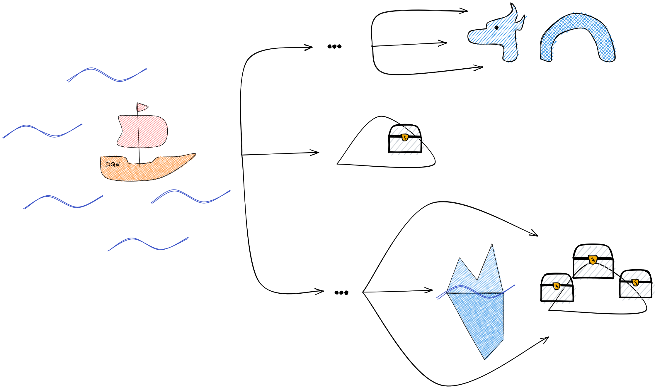
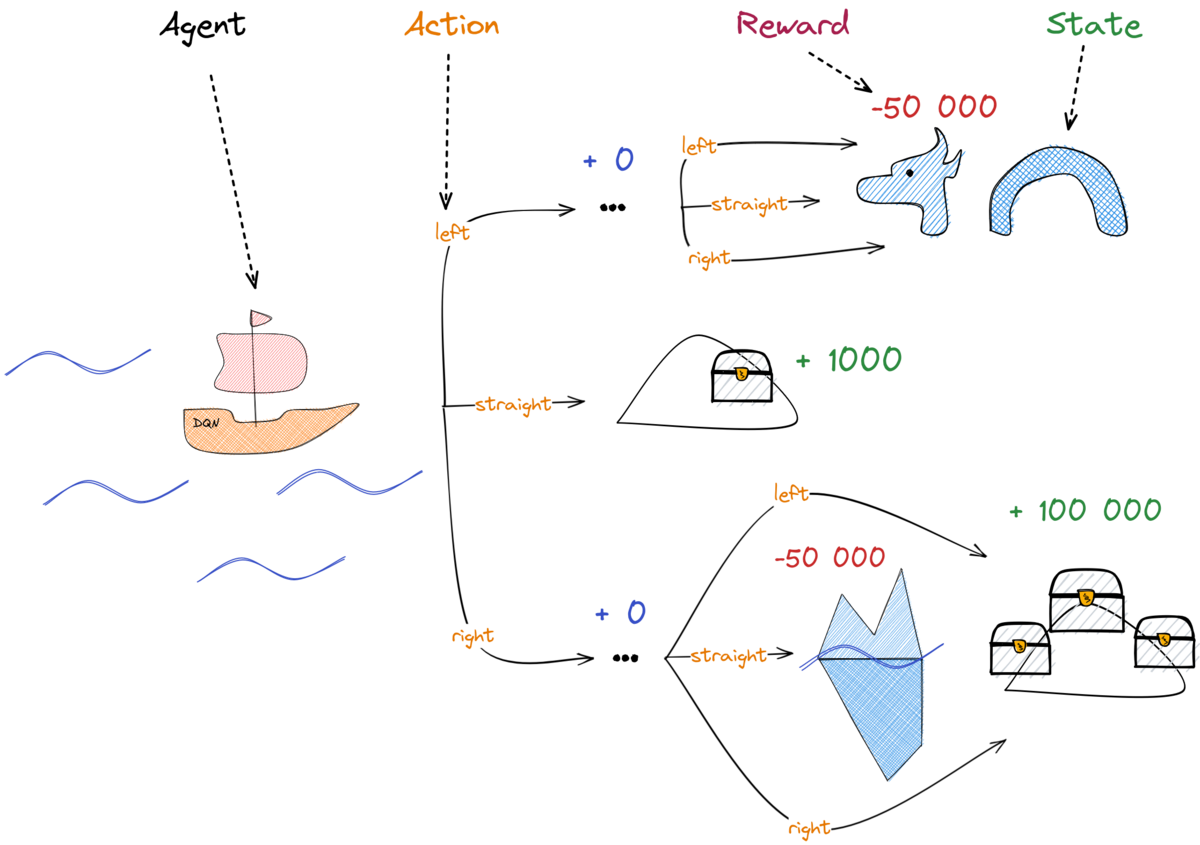
- Agent: the "boat", our main character
- State: Where are we? (position, speed, ...)
- Action: What can we do? (steer left, right, ...)
- Reward: How good are we doing?
- Policy: The "captain", defines the agent's behavior
Value Functions
How good is it to be in this state?
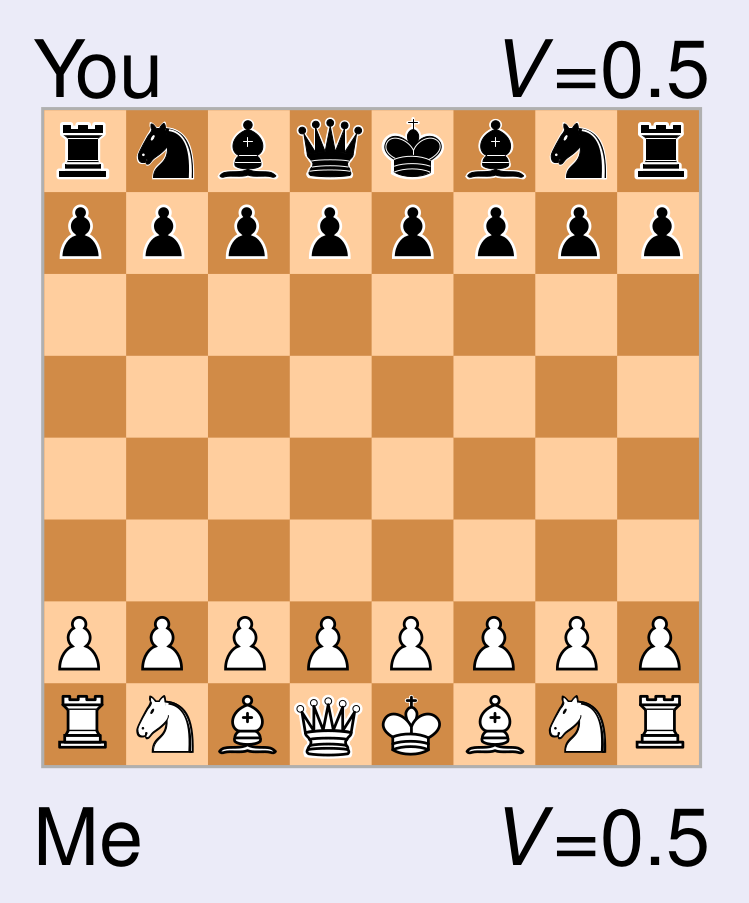
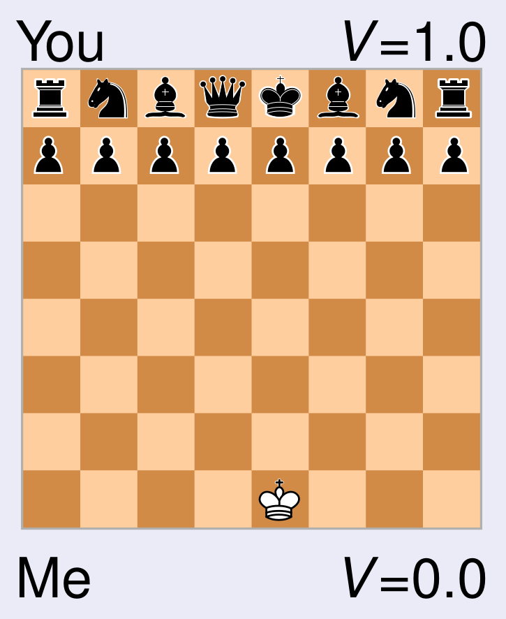
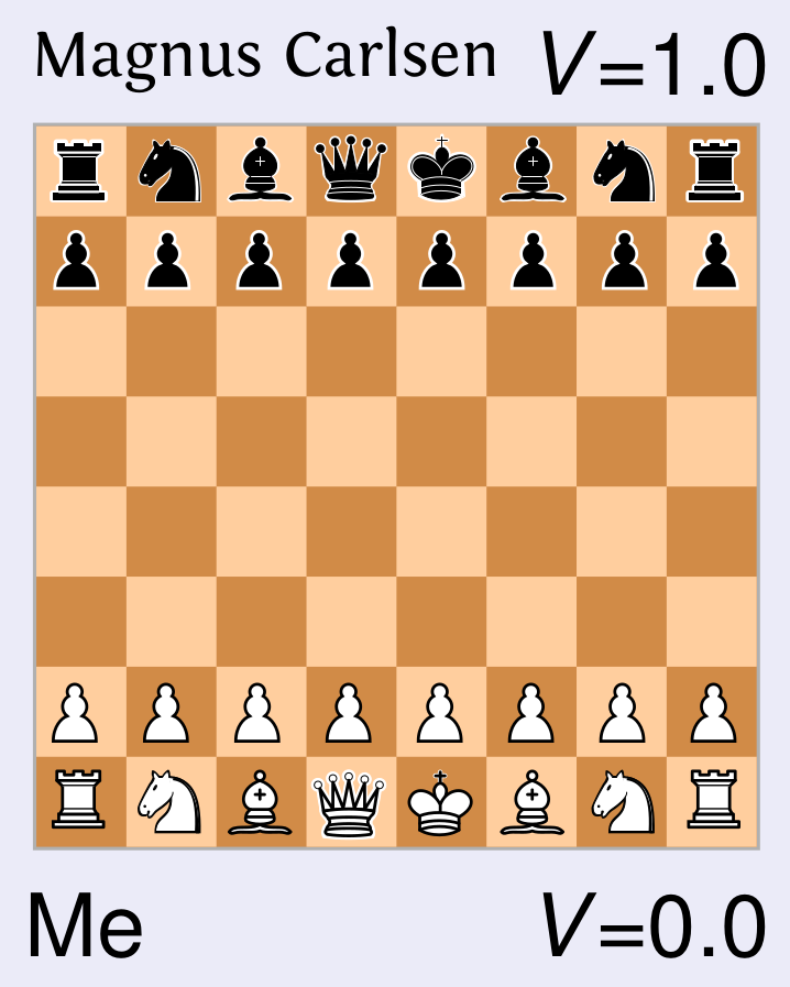
Win: 1.0 | Draw: 0.5 | Lose: 0.0
Depends on the state
Depends on the policy
Source: Freek Stulp - Master AIC
Action-Value Function: Q-Value
What if we have no model?
Solution: $Q_\pi(s, a)$ instead of $V_\pi(s)$
\[\begin{aligned} \pi(s) = \argmax_{a \in A} Q_\pi(s, a) \end{aligned} \]
Tabular Q-Learning: Discrete States
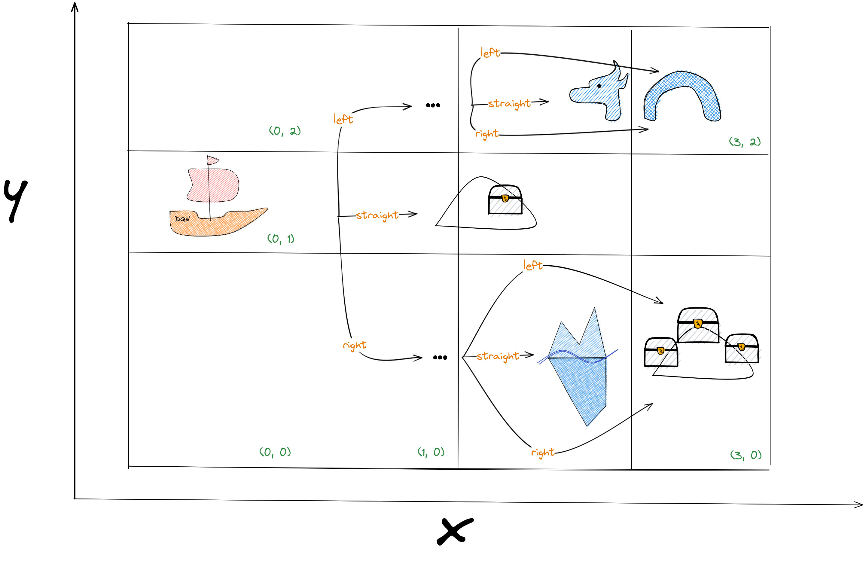
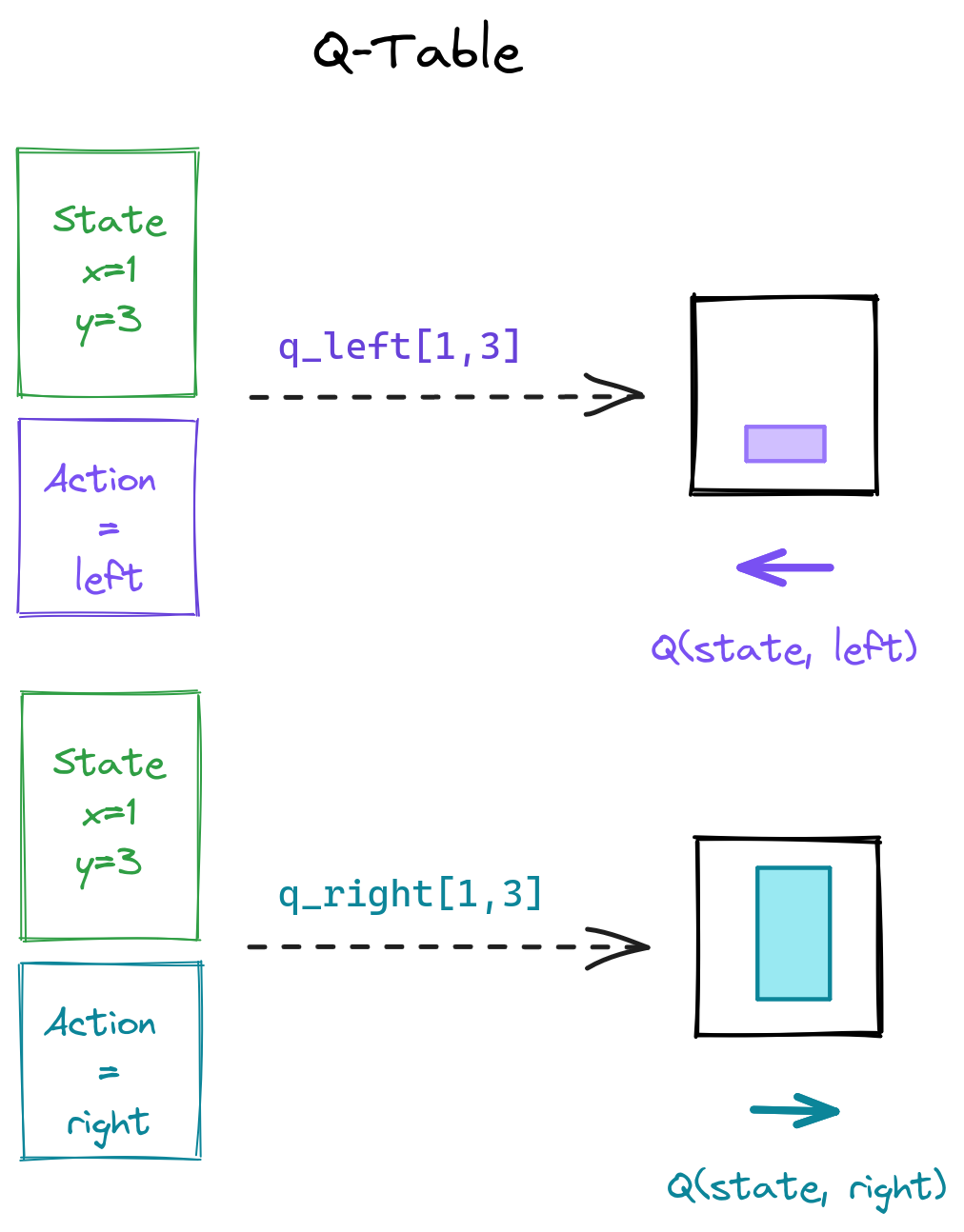
Tabular Q-Learning: Q-table
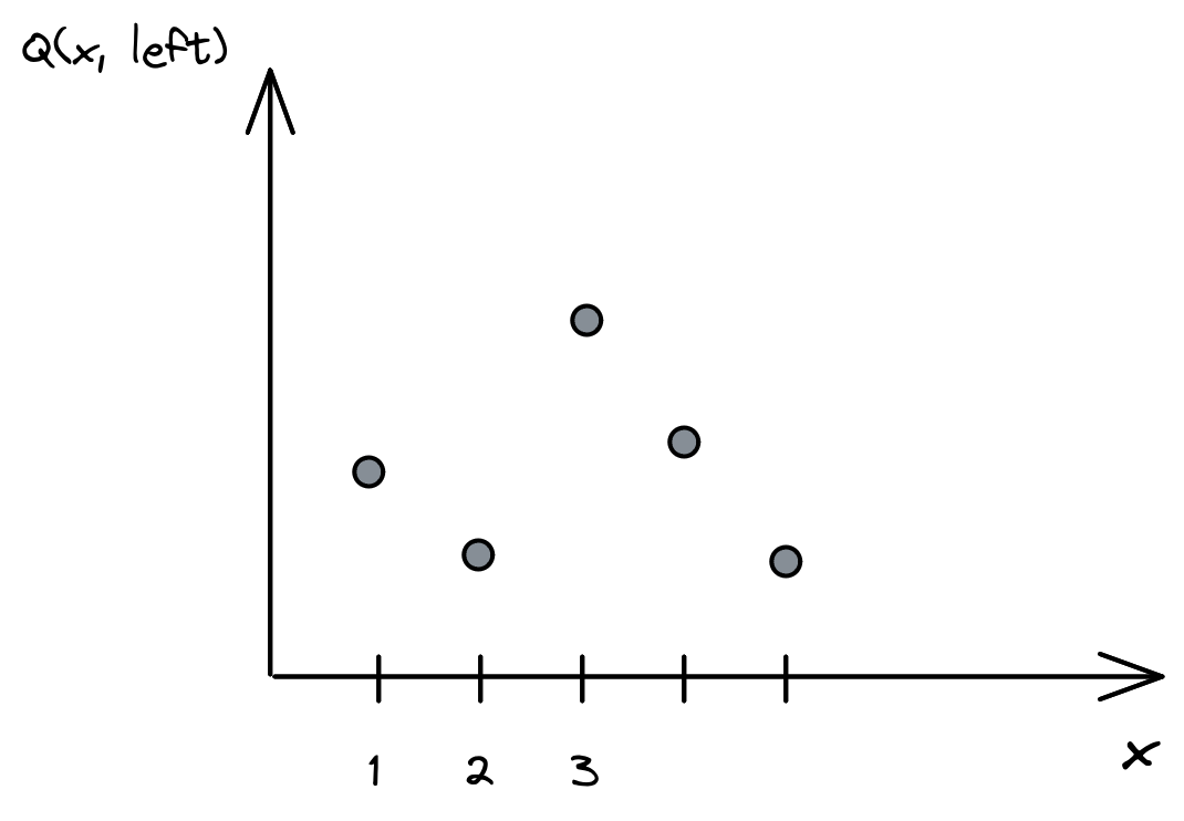
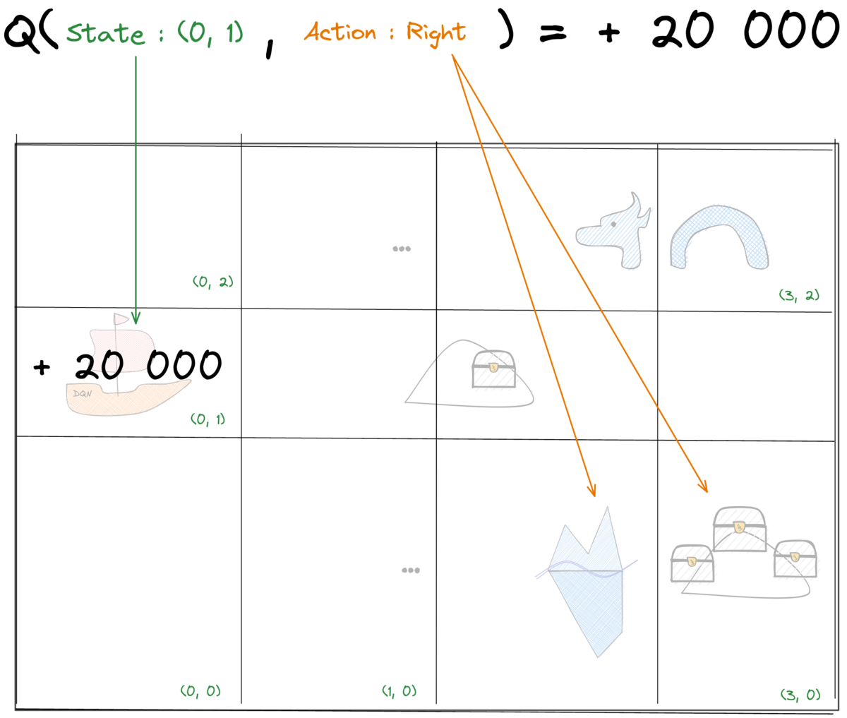
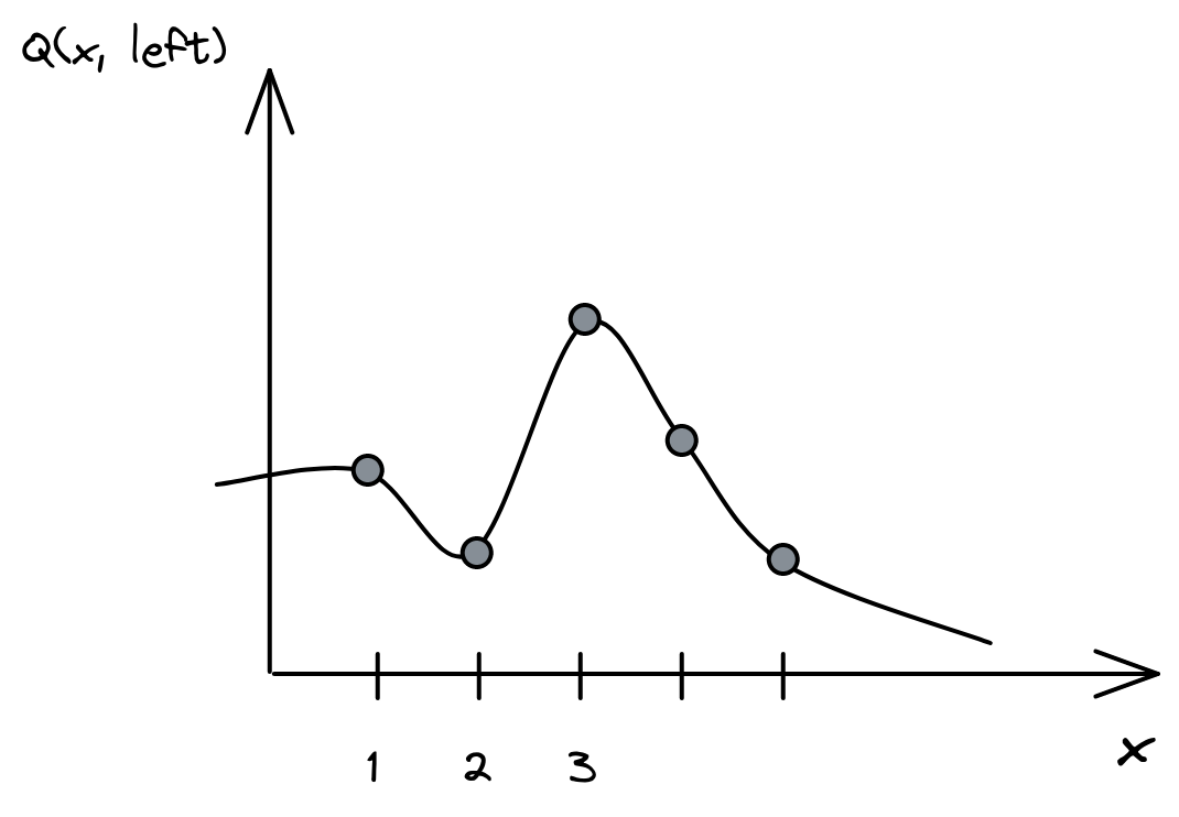
Tabular Q-Learning: Q-values
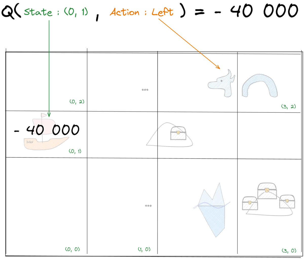
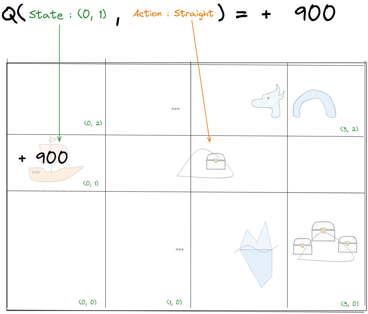
Tabular Q-Learning: Update rule
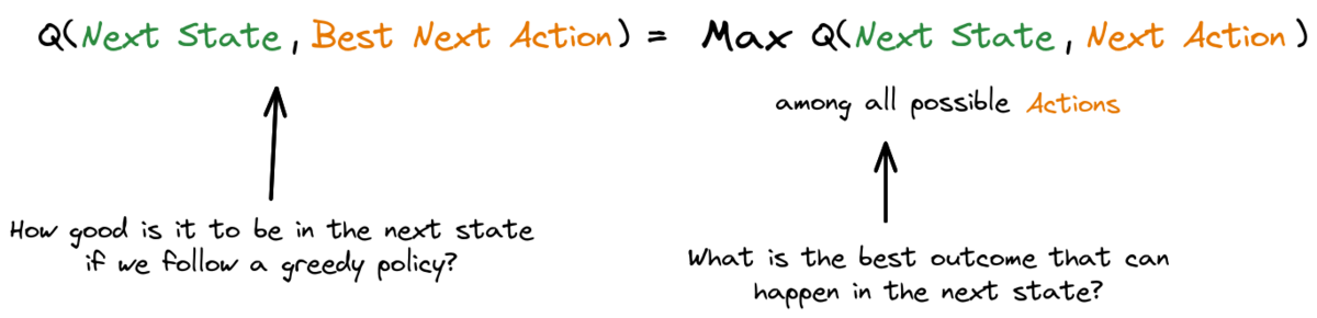
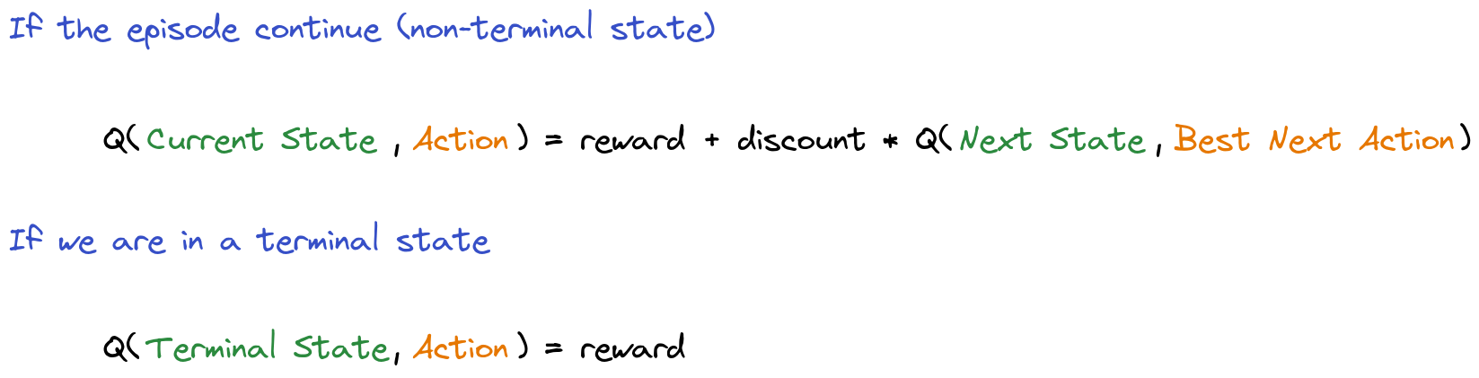
Bellman equation for optimal value function:
Q-learning update rule
Tabular Q-Learning: Update explained
$\alpha=1$ (learning rate)

Reminder

Tabular Q-Learning: Terminal State
Questions?
Tabular Q-Learning: Limitations
- Discrete states
- No generalization (lookup table)
- Discrete actions
How to go beyond tabular Q-Learning?
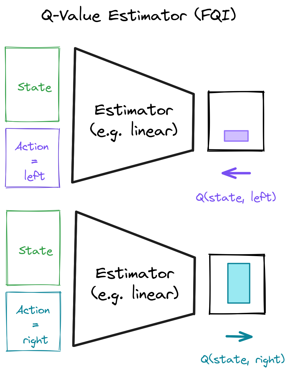
Q-Value Estimator
Q-Learning Regression (1/2)
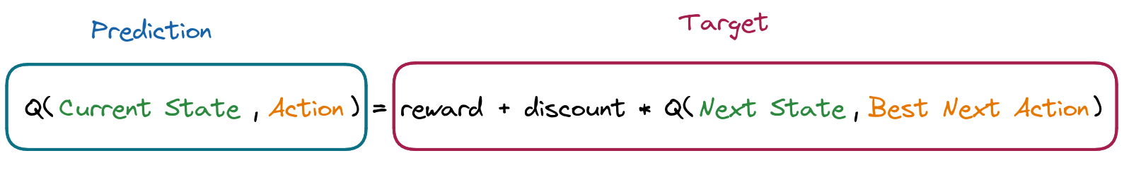
One small detail...
$\textcolor{#1864ab}{Q_\theta(s_t, a_t)}$ depends on $\textcolor{#a61e4d}{Q_\theta(s_{t+1}, a')}$...
What can we do about it?
Iterate! Use $Q^{\textcolor{green}{n}}_\theta(s_t, a_t)$
Fitted Q-Iteration (FQI) (1/2)
- Create the training set based on the previous iteration $ Q^{\textcolor{green}{n-1}}_\theta(s, a) $ and the transitions:
- input: $\textcolor{#1864ab}{x = (s_t, a_t)}$
- if $s_{t+1}$ is non terminal: $y = r_t + \gamma \cdot \max_{a' \in A}(Q^{n-1}_\theta(s_{t+1}, a'))$
- if $s_{t+1}$ is terminal: $\textcolor{a61e4d}{y = r_t}$
- Fit a model using a regression algorithm to obtain $ Q^{\textcolor{green}{n}}_\theta(s, a) $
\[\begin{aligned} \textcolor{#1864ab}{f_\theta(x)} = \textcolor{#a61e4d}{y} \end{aligned} \]
- Repeat, $\textcolor{green}{n = n + 1}$
Fitted Q-Iteration (2/2)
- $\textcolor{#1864ab}{x = (s_t, a_t)}$
- $\textcolor{#a61e4d}{y = r_t}$
Fitted Q-Iteration (code)
									initial_targets = rewards
									# Initial Q-value estimate
									qf_input = np.concatenate((states, actions))
									qf_model.fit(qf_input, initial_targets)

									for _ in range(N_ITERATIONS):
									    # Re-use Q-value model from previous iteration
									    # to create the next targets
									    next_q_values = get_max_q_values(qf_model, next_states)
									    # Non-terminal states target
									    targets[non_terminal_states] = rewards + gamma * next_q_values
									    # Special case for terminal states
									    targets[terminal_states] = rewards
									    # Update Q-value estimate
									    qf_model.fit(qf_input, targets)
CartPole Env
https://gymnasium.farama.org/environments/classic_control/cart_pole/
Gym/Gymnasium API
							 import gymnasium as gym

							 # Create the environment
							 env = gym.make("CartPole-v1", render_mode="human")
							 # Reset env and get first observation
							 obs, _ = env.reset()

							 # Step in the env with random actions and display the env
							 for _ in range(100):
							     env.render() # Display the env

							     action = env.action_space.sample()
							     # Retrieve new observation, reward,
							     # termination signal, truncation signal
							     # and additional infos
							     next_obs, reward, terminated, truncated, info = env.step(action)
							     # Update current observation
							     obs = next_obs
							     # End of an episode
							     if terminated or truncated:
							         obs, _ = env.reset()
FQI in practice (1st notebook)
FQI Limitations
- Offline RL
- Loop over all possible actions $A$ to get next best action $\textcolor{#a61e4d}{a'}$: \[\begin{aligned} \max_{\textcolor{#a61e4d}{a' \in A}} Q_\theta(s_{t+1}, \textcolor{#a61e4d}{a'}) \end{aligned} \]
- Instability (target depends on $Q^{n-1}_\theta(s_{t+1}, a')$)
From FQI to DQN
- Offline RL → Online RL
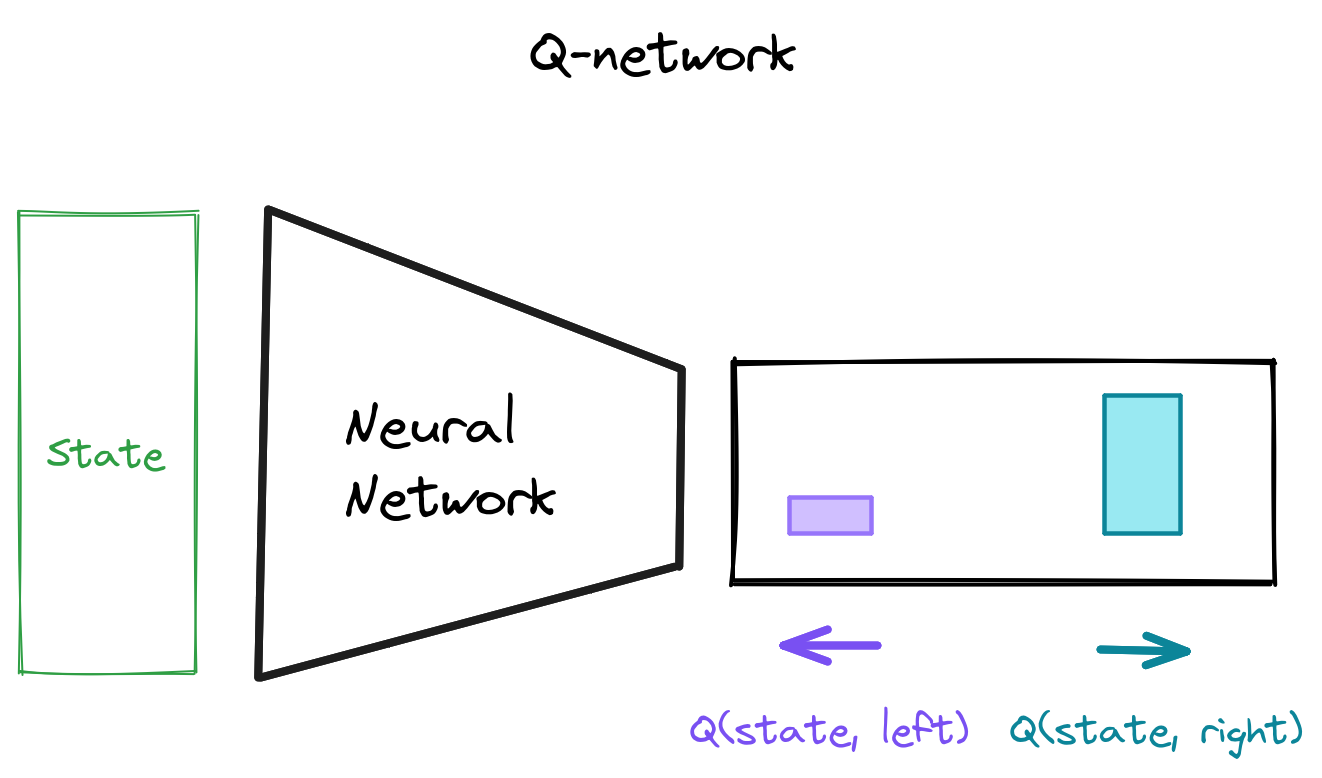
- Loop over actions → One forward pass to get all $Q_\theta(s, a)$
- Instability → Target Network $Q_{\textcolor{green}{\theta'}}(s, a)$
Questions?
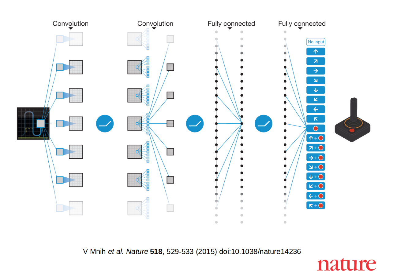
Deep Q-Network (DQN)
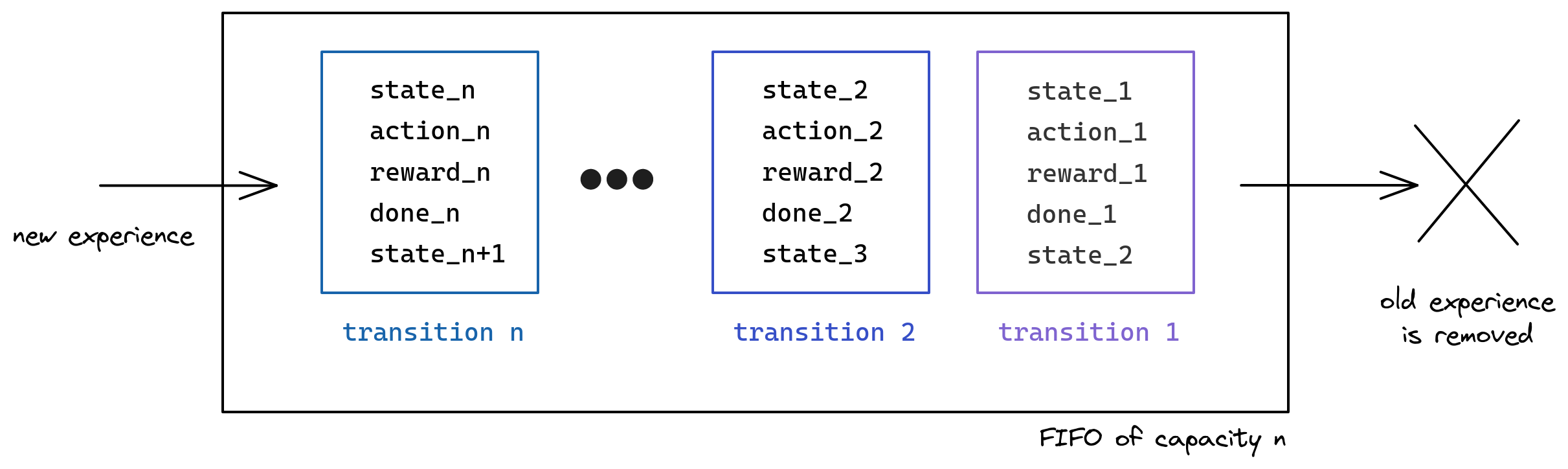
Replay Buffer
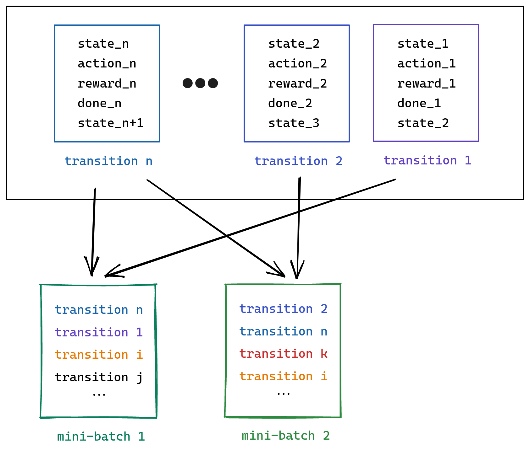
Replay Buffer Sampling
Q-network
The training loop

Collecting Experience
								# Retrieve q values for the current observation
								q_values = q_model(current_obs)

								# Follow greedy-policy:
								# take the action with the highest q_value
								action = np.argmax(q_values)

								# Do one step in the env
								next_obs, reward, terminated, _, _ = env.step(action)

								# Store transition in the replay buffer
								replay_buffer.store(obs, action, reward, terminated, next_obs)
Exploration / Exploitation
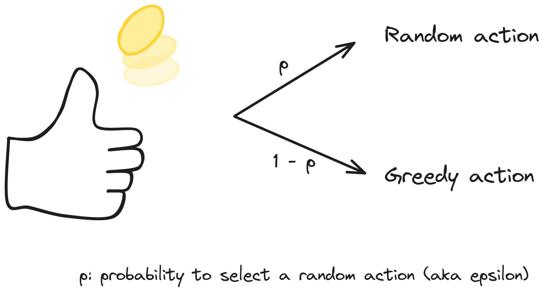
Epsilon-greedy Exploration
							 # Flip a biased coin
							 take_random_action = np.random.rand() < exploration_rate

							 if take_random_action:
							     # Random action
							     action = action_space.sample()
							 else:
							     # Greedy action
							     action = np.argmax(q_values)
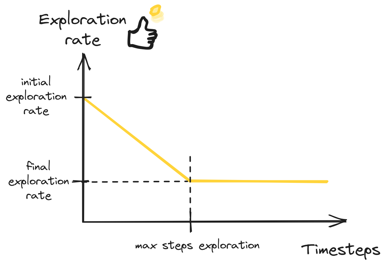
Exploration Schedule
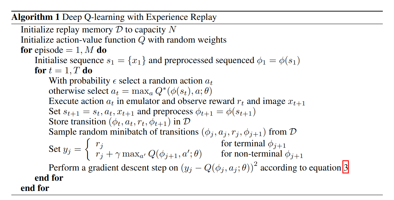
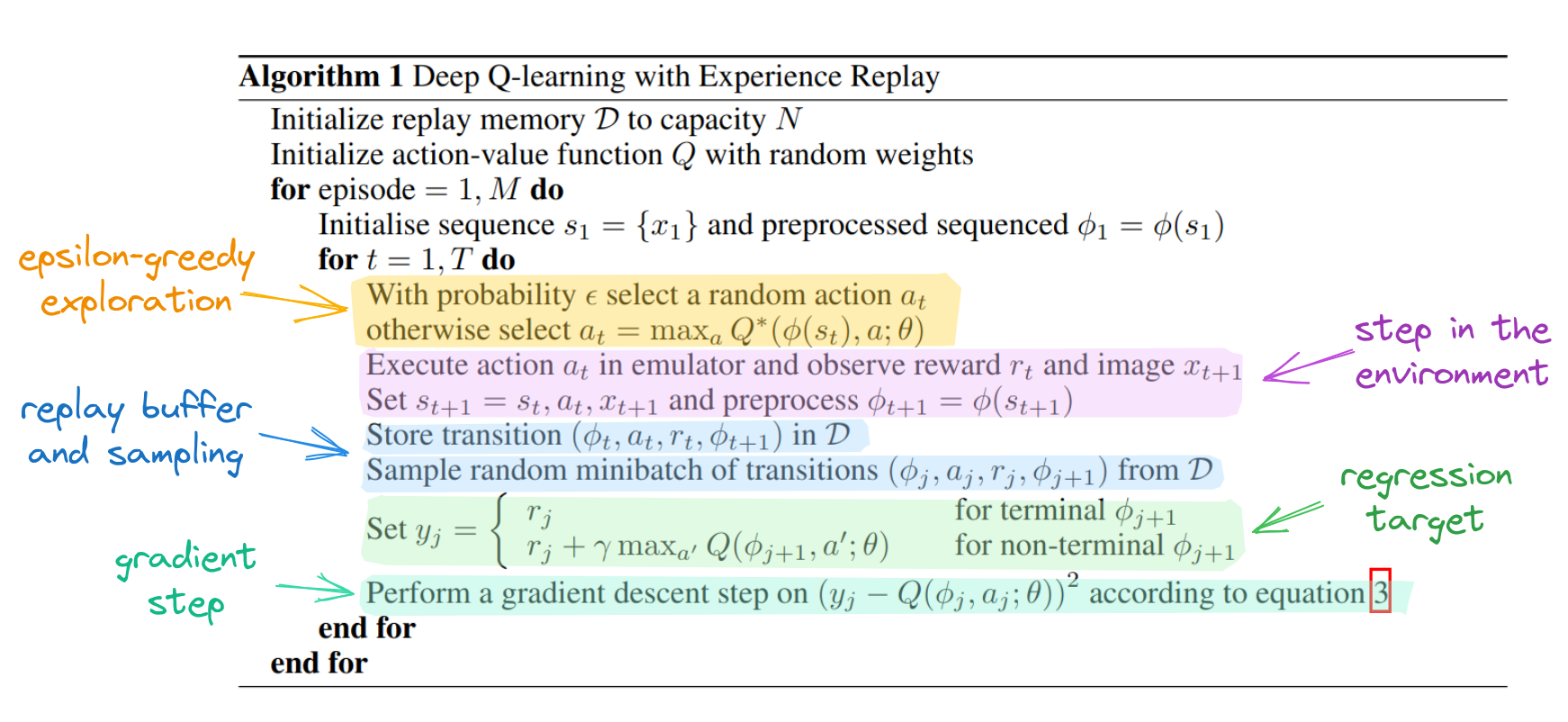
Annotated DQN Algorithm
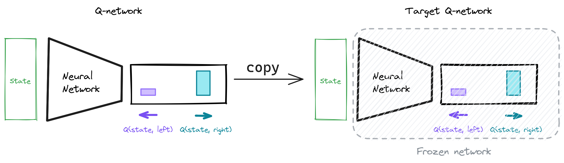
Target Q-Network
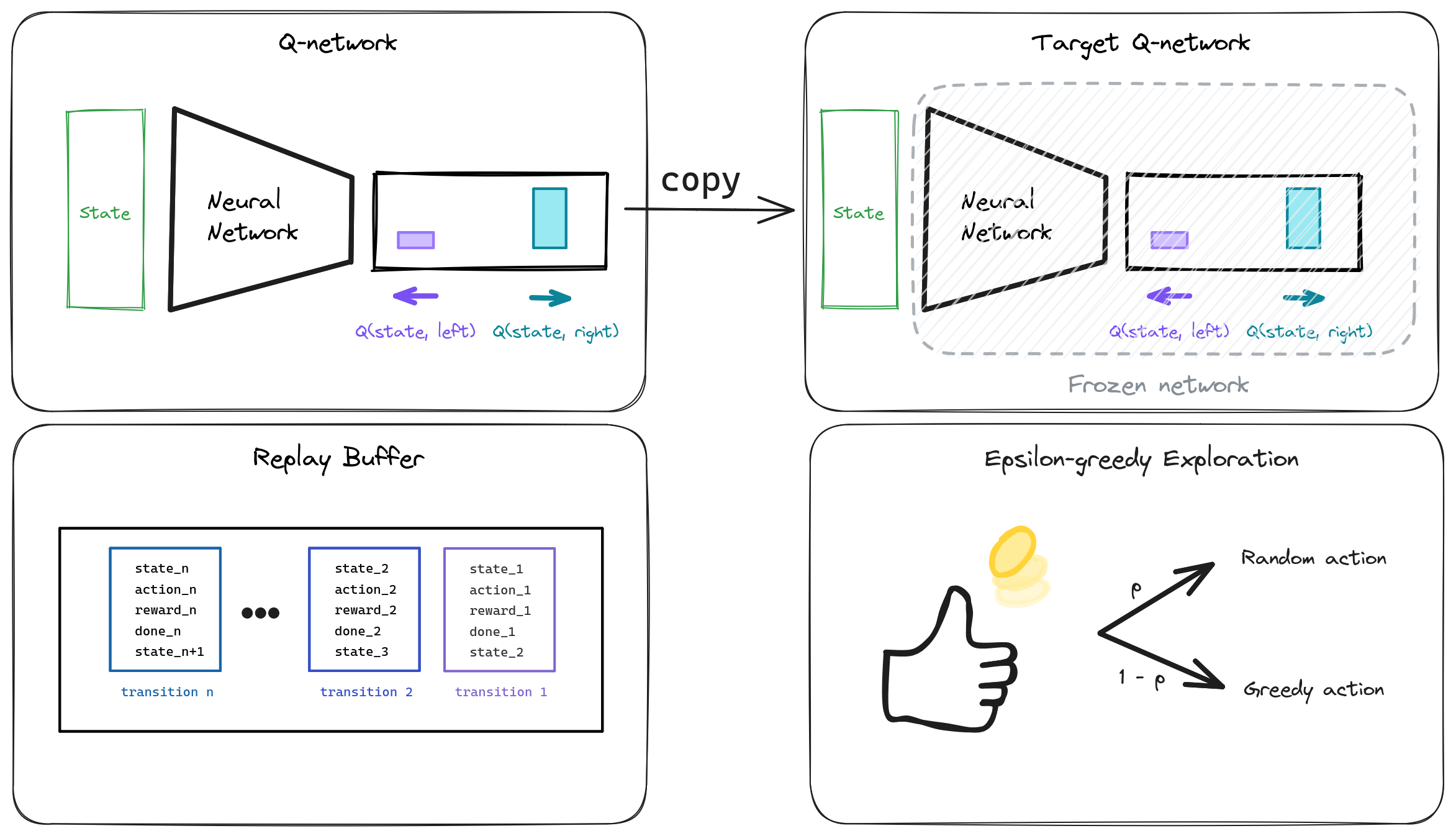
DQN Overview
Questions?
PyTorch API
| NumPy | PyTorch |
|---|---|
np.array([[1, 2], [3, 4]]) |
th.tensor([[1, 2], [3, 4]]) |
np.ones((2, 3)) |
th.ones(2, 3) |
np.concatenate |
th.cat |
x.shape |
x.shape |
x.argmax(axis=...) |
x.argmax(dim=...) |
x.item() |
x.item() |
| NumPy to PyTorch: | th.as_tensor |
Backup Slides
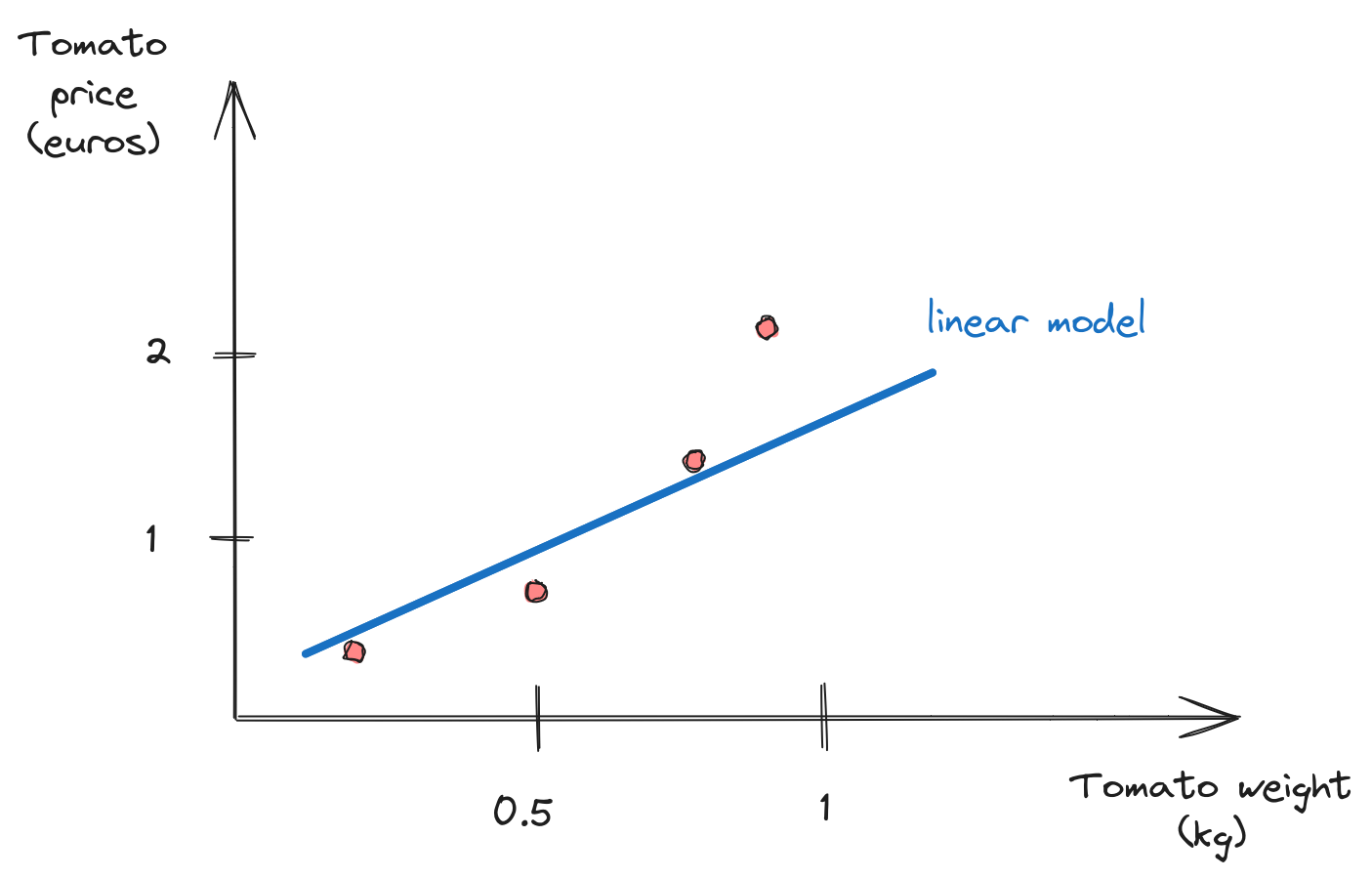
Regression 101
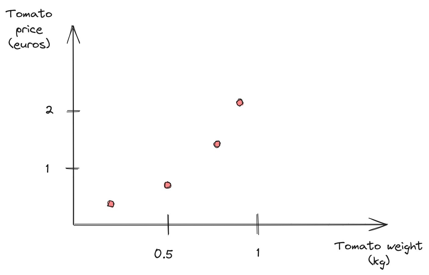
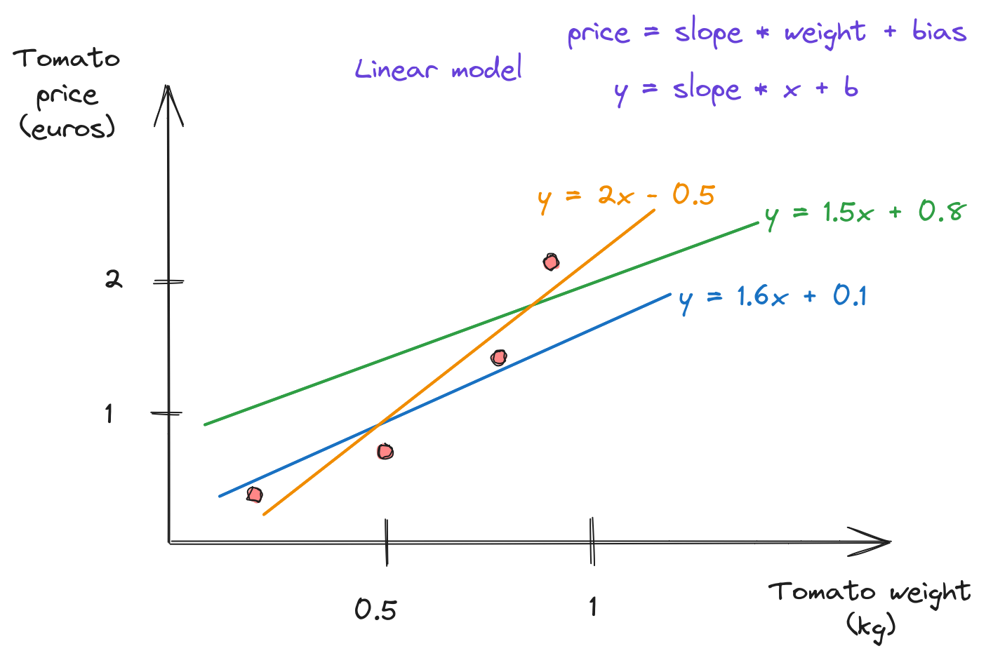
Linear model
Linear model(s)?
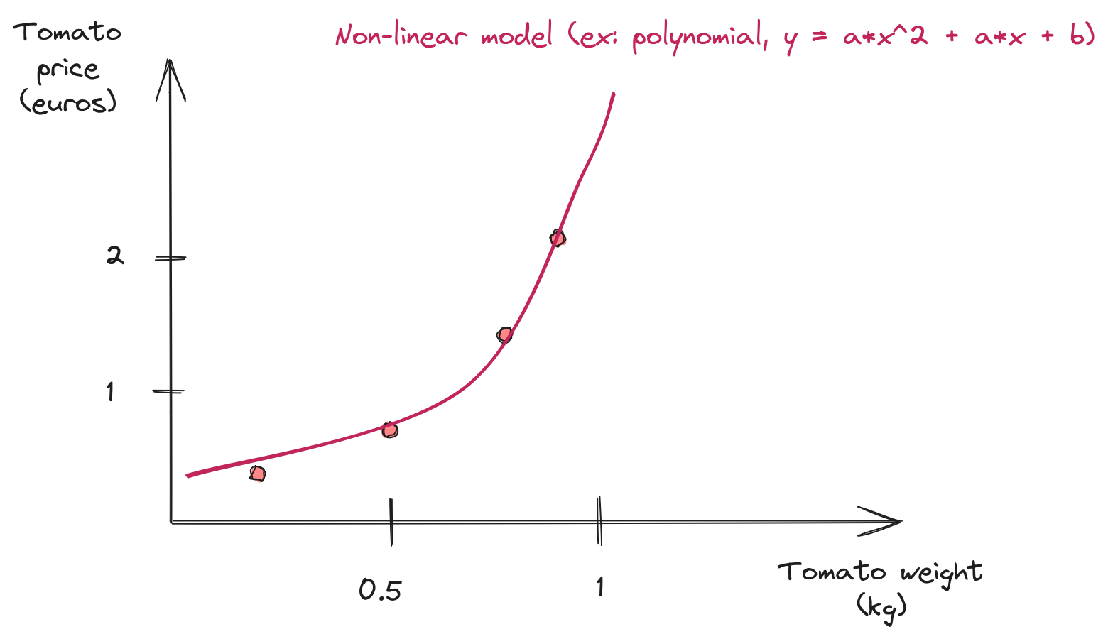
Non Linear Model
Scikit-Learn API
								import numpy as np
								from sklearn.linear_model import LinearRegression
								# Generate some data (noisy linear function)
								x = np.linspace(0, 5, num=50).reshape(50, 1)
								y = 2 * x + 10 + 0.1 * np.random.rand()
								# Fit a linear model using least squares
								model = LinearRegression().fit(x, y)
								y_predict = model.predict(x)
								# Retrieve the optimized parameters
								slope, bias = model.coef_, model.intercept_